"Stochastics as Physics": Completing the mathematical part

Preview of Chapters 3 and 4 of my book in preparation

This is the third post about my book in preparation “Stochastics as Physics”. The two earlier posts are linked below.

Introducing "Stochastics as Physics"

Probability theory in "Stochastics as Physics"

I have now completed Chapters 3 and 4. I am not that quick as it may seem: These chapters were almost ready in my other book I presented before.

Stochastics of Hydroclimatic Extremes - A Cool Look at Risk: Edition 5

I only had to make some adaptations for the context of stochastics as physics.

So here is the current book version with four chapters ready. The new chapters 3 and 4 are entitled, respectively “Stochastic processes and quantification of change” and “Fundamental concepts of statistics and their adaptation to stochastic processes”.

Stochastics as Physics With Applications to Geophysics and Engineering

3.99MB ∙ PDF file

Download

Chapters 1 to 4

Download

Like chapter 2, the new chapters are heavy in terms of math, but hopefully self-contained. Those unfamiliar with my other book will find the content of these chapters quite novel: I am not copying textbooks; rather I compile my own (and my colleagues’) several works in a stand-alone style. The next chapters are planned to contain more physics and geophysics and less math.

For this post I chose to copy one Digression from each of the two chapters, which contain lighter material, perhaps being more useful than the heavy material.

---

Digression 3.B: What is dependence in time?

Dependence can be simply defined as the absence of independence. With reference to equation (2.5) defining independence and using equations (3.2)–(3.4), we define dependence in a stochastic process in time (also known as intertemporal dependence or simply time dependence) by

\( F(x_1,x_2,…,x_n;t_1,t_2,…,t_n )≠F(x_1;t_1 )F(x_2;t_2 )⋯F(x_n;t_n ) \)

It is typically expressed by the autocovariance or the autocorrelation function and its typical (mis)interpretation is memory. This has been so common that in many texts the term memory has replaced the term dependence—even in the titles of several publications, papers and books. Perhaps the scientist who was most influential in establishing this interpretation was Mandelbrot (for example, Mandelbrot and Wallis, 1968,¹ speak about short and long memory, both of which they contrast to independence), though other scientists had used the term before (e.g. Krumbein, 1968)². Clearly, in stochastics the term memory is metaphorical, while in other disciplines (neuropsychology, computer science) it is literal. In science there is no reason to use a metaphorical term when we have a literal term, particularly when the metaphorical term has another scientific meaning. The use of the metaphorical term memory distracts, rather than helps, intuition and the understanding of time dependence in a stochastic process. In particular, the use of its variant long memory is totally inappropriate as it stimulates people to imagine a mechanism inducing long memory (e.g. hundreds of years) and of course it is difficult to conceptualize such a mechanism. A better interpretation is a mechanism that produces change, rather than one that recalls information (as is the meaning of memory). And indeed, changes produce dependence—not the other way round. Furthermore, dependence and change need not be interpreted as nonstationarity as many think.

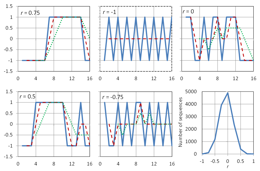
Before discussing how change produces time dependence in a process that is stationary, we will discuss how dependence manifests itself into a time series. In one word, this manifestation is through patterns. In pure randomness, without time dependence (like in a sequence of dice outcomes or in the sequence of digits of π) no patterns appear. To better illustrate such patterns, we examine several time series with a small length, n = 16. For convenience we make these time series two-valued, with values –1 and 1 and with an average of the 16 values equal to zero, which means that eight values will be –1 and eight 1. The estimates of the variance, the lag-one autocovariance and the lag-one autocorrelation coefficient will thus be, respectively:

\(\hat{\gamma }_1=\frac{1}{16} \sum _{\tau =1}^{16} x_{\tau }^2=1,\text{ }\text{ }{\hat{c}_1=\frac{1}{16} \sum _{\tau =1}^{16} x_{\tau } x_{\tau +1}}, \text{ }{\hat{r}_1=\frac{\hat{c}_1}{\hat{\gamma }_1}=\hat{c}_1}\)

where we set x₁₇ = x₁ in order to have 16 terms in the sum for c ̂₁ and thus make possible values up to ±1. (Note, though, that this practice is not being suggested to use in analyses of time series). The formal meaning of the term estimate is clarified in section 4.3.

Examples of such time series are shown in Figure 3.2. In the upper left panel, all eight ones are grouped together so that

\({\sum _{\tau =1}^{16} x_{\tau } x_{\tau +1}=7+7-2=12}\)

and r ̂₁ = 0.75. This is the highest possible value that a particular arrangement of 16 items, each being ±1, can give. Obviously, there are 16 possible arrangements that will give r ̂₁ = 0.75. If our time series had length N, the highest r ̂₁ would be (N — 4) / N = 1 — 4/N, and would approach the value +1 for large N. Consequently, a large autocorrelation is caused by grouping together of similar (in our example, the same) values. Such grouping has been termed persistence. If the grouping appears but is not that “perfect”, such as in the lower left panel, then again, the autocorrelation will be positive but lower (r ̂₁ = 0.5 in this example).

In contrast, if the patterns appear to be of alternating, rather than grouping, type, then the autocorrelation coefficient is negative. Thus, in the “perfect” alternating shape of the upper middle panel of Figure 3.2 we have that

\({\sum _{\tau =1}^{16} x_{\tau } x_{\tau +1}=-1}\)

and hence r ̂₁ = —1. In the lower middle panel, alterna­tion is not perfect and r ̂₁ = —0.75. Finally, the upper right panel is free of patterns and r ̂₁ = 0.

Now, the effect of change is illustrated in Figure 3.3, where we plot a time series generated from the normal distribution without time dependence. We now assume that the process is affected by a mechanism producing change, namely shifts up and down, at random points in time. As illustrated in Figure 3.3 and detailed in the figure caption, in this case patterns are produced and (positive) autocorrelation is induced.

Figure 3.2 Examples of arrangements of eight ones and eight minus ones in the form of time series with length 16, mean zero and unit variance, along with the resulting estimate of the lag-one autocorrelation coefficients r. In addition to the original time series (scale 1; continuous line), time-averaged time series are also shown at scales 2 (dashed lines) and 4 (dotted lines). In the bottom right panel, the frequency distribution of r for all 16! / (8!)² = 12 870 possible cases (permutations) are shown.

Figure 3.3 Illustration of the fact that change causes autocorrelation using a time series of length 20, generated from the normal distribution N(0,1) without time dependence; the estimates of the statistical characteristics from the time series, plotted as full points connected with continuous lines, are μ ̂ = —0.05, γ ̂₀ = 0.9², r ̂₁ = 0.05. By shifting a time segment up (by +1, items 8-14) and another segment down (by –1, items 15-20) we obtain a new time series (empty points connected with dashed lines) in which the autocorrelation has become r ̂₁ = 0.59.

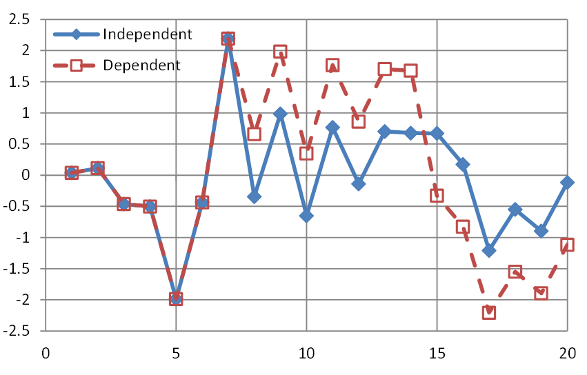
Had such change been describable in deterministic terms, as a deterministic function of time, that is, had it been precisely predictable in terms of location of times where it occurs and in terms of magnitude of state shifts, we would speak about nonstationarity. But since, as we said, the points of change are random points in time, they resist a deterministic description and the entire process with the change-producing mechanism is a stationary stochastic process with dependence. Unfortunately, this simple truth is not widely understood and therefore the inconsistent interpretations of change as nonstationarity abound in geophysics literature.

---

Digression 4.A: Deduction and induction

The theory of probability has provided solid scientific grounds for philosophical concepts such as indeterminism and causality. In many scientific and technological applications, probability has provided the tools to quantify uncertainty, rationalize decisions under uncertainty, and make predictions of future events under uncertainty, in lieu of unsuccessful deterministic predictions (see Koutsoyiannis, 2010)³.

Probability has also provided the basis for extending the typical mathematical logic, offering the mathematical foundation of induction. Thus, probability made it possible to incorporate into mathematics the entire Aristotelian logic, which in addition to deductive reasoning or deduction (the Aristotelian apodeixis) also includes induction (the Aristotelian epagoge).

Ἀριστοτέλης (Aristotle; 384–322 BC), Greek philosopher of the Classical period, founder of the Lyceum and the Peripatetic School of philosophy. (Image source: Visconti, E.Q., 1817: Planches de l’Iconographie Grecque. De l’Imprimerie de P. Didot l’Ainé, Paris, 58 plates—engravings, https://archive.org/ details/gri_33125010850713/ and https://arachne.dainst.org/entity/1884649).

In classical mathematical logic, determinism can be paralleled to the premise that all truth can be revealed by deductive reasoning. This type of reasoning consists of repeated application of strong syllogisms concerning the logical propositions A and B, such as:

Case 1

• (Premise): If A is true, then B is true;

• (Evidence): A is true;

• (Conclusion): B is true.

Case 2

• (Premise): If A is true, then B is true;

• (Evidence): B is false;

• (Conclusion): A is false.

Deduction uses a set of axioms to prove propositions known as theorems, which, given the premises (based on axioms), are irrefutable, absolutely true statements. It is also irrefutable that deduction is the preferred route to truth. The question is, however, does deduction have any limits?

David Hilbert’s famous aphorism “Wir müssen wissen, wir werden wissen” (“We must know, we will know”; see section 1.1), expressed his belief that there were no limits to deduction. According to this belief, more formally known as completeness, any mathematical statement could be proved or disproved by deduction from axioms. However, developments in mathematical logic, and particularly Gödel’s incompleteness theorem, challenged the omnipotence of deduction suggesting the usefulness and necessity of induction.

Induction uses weaker inference rules of the type:

Case 3

• (Premise): If A is true, then B is true;

• (Evidence): B is true;

• (Conclusion): A becomes more plausible.

Case 4

• (Premise): If A is true, then B is true;

• (Evidence): A is false;

• (Conclusion): B becomes less plausible.

Induction offers no proof as to whether a proposition is true or false and may lead to errors. However, it is very useful in decision making, when deduction is not possible, which is the case quite frequently in the real world and everyday life (see Jaynes, 2003)⁴.

The important achievement of probability is that it quantifies (expresses in the form of a number between 0 and 1) the degree of plausibility of a certain proposition or statement. The formal probability framework uses both deduction, for proving theorems, and induction, for inference with incomplete information or data. For the latter we use the branch of stochastics called statistics.

Your comments will be most welcome
as they help me improve the material I am presenting.

1. Mandelbrot, B.B. and Wallis, J.R., 1968. Noah, Joseph, and operational hydrology. Water Resources Research, 4(5), 909-918.

2. Krumbein, W.C., 1968. Statistical models in sedimentology. Sedimentology, 10 (1), 7-23.

3. Koutsoyiannis, D., 2010. A random walk on water. Hydrology and Earth System Sciences, 14, 585–601, doi: 10.5194/hess-14-585-2010.

4. Jaynes, E.T., 2003. Probability Theory: The Logic of Science, Cambridge Univ. Press, Cambridge, UK, 728 pp.